This post will discuss a simple method for land cover classification using a k-means clustering algorithm with Spectral Python (SPy). Spectral is a pure-Python package for processing hyperspectral images and is available for download using Pip or Conda.
Let’s say you are working on a suitability analysis project and want to include the land cover as a layer in the model. I know there are data in the public domain for land cover classification, but wouldn’t it be nice if we can generate our own using more recent imagery. Public land cover data are available for the Conterminous US via the National Land Cover Database (NLCD CONUS land cover data). NLCD data is updated only every 2-3 years, so it is handy to make your own rough classifications using Landsat 8 imagery. In most cases, Landsat 8 visible bands (bands 2, 3, and 4) are sufficient for a landscape level analysis.
The k-means algorithm for unsupervised classification in Spectral Python is easily accessed via a Python function. A sample call to the function kmeans is shown below. This example would create 20 clusters (classes) using 30 iterations. The data is provided as a variable ‘img’, which is an n-dimensional array (NumPy).
(m, c) = spectral.kmeans(img, 20, 30)The land cover map below was generated using the default parameters, and identifies 10 unique clusters (i.e. classes). The area outlined in black is the Area of Interest (AOI) for this analysis. Typically I would clip the raster output to the AOI, but I wanted to see how the classification performed overall.
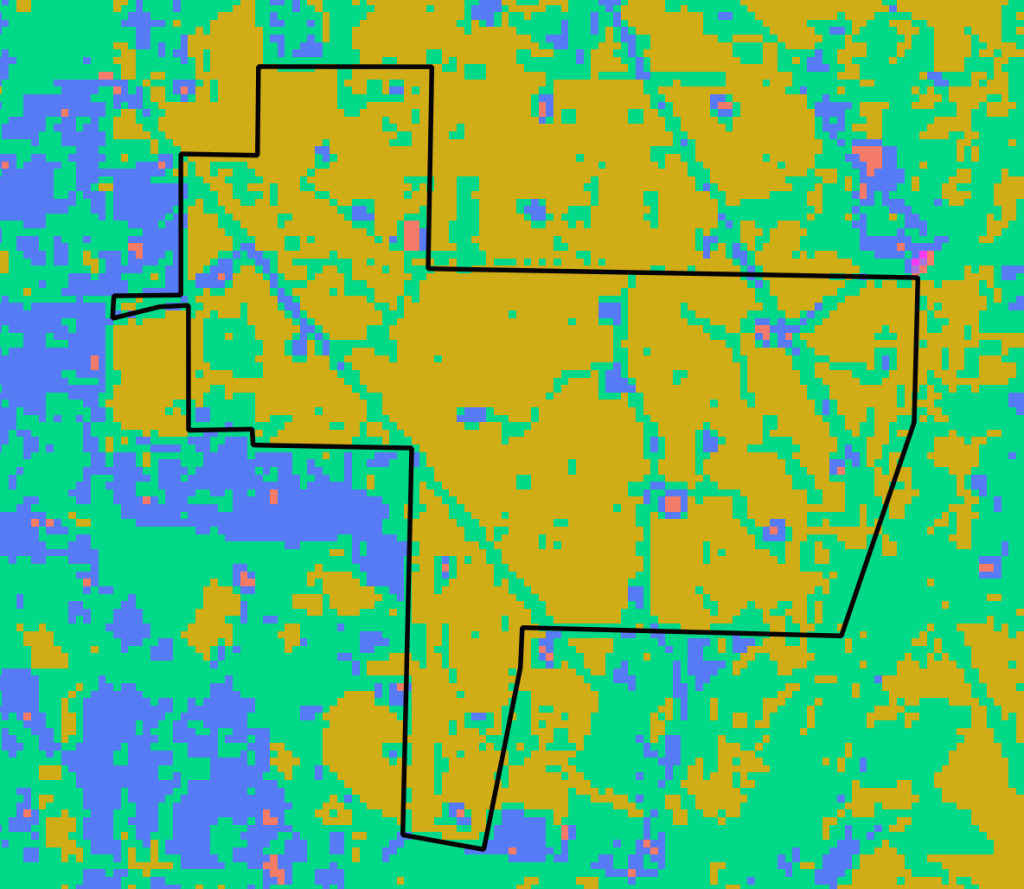
The resulting output above is not perfect, but its pretty good. The yellow pixels represent evergreen forest type. The teal green pixels represent open areas (pastures, utility ROWs, etc), but also includes some deciduous forest types that were misclassified. The blue pixels represent developed areas like well sites and lease roads. However, some of the blue areas were actually misclassified fields and pastures. Its not a perfect model, but in many cases these results may be good enough for a quick analysis.
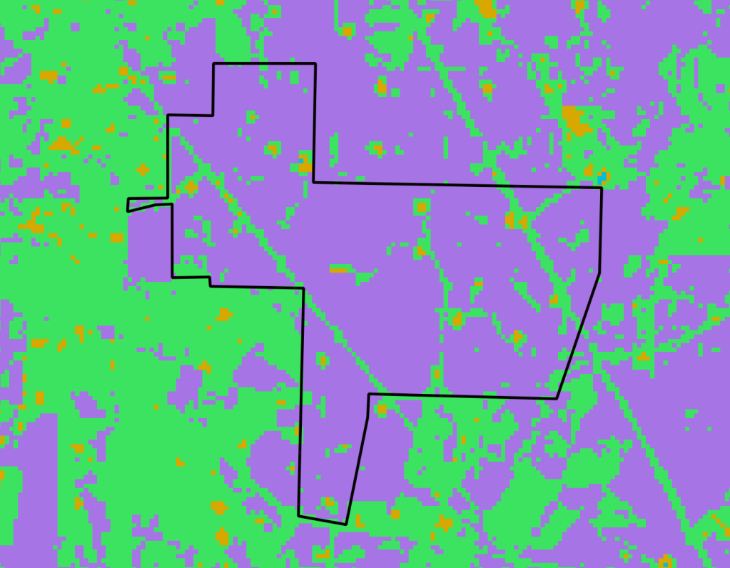
The following image shows another classification attempt using 5 classes and 20 iterations. This time the model performed a little better on the open areas and young planted pine forests. Purple pixels represent forested areas (pine and hardwood) and green pixels represent developed areas like roads and well sites, but also includes fields and pastures. Bare ground and highly reflective areas are represented by orange pixels. A drawback of this run is that the young forested areas (<5 years old) were classified with the open areas. However, tweaking the model parameters or using more image bands may provide better results.
There were some misclassifications using this approach, but overall it performed pretty well for an unsupervised classification with very little effort required. I’m guessing that it is around 75-85% accurate using the default parameters, and maybe as much as 85-90% accurate through trial and error. The good news is the model is simple and we can easily change parameters and visualize the results.
A complete example of how to perform k-means classification, and other examples of working with raster data, can be found in Chris Garrard’s book “Geoprocessing with Python” published by Manning. This is a good reference for anyone wanting to learn geospatial Python. I highly recommend it.
Post Photo by Benjamin Cheng on Unsplash
Categories: Forestry Apps